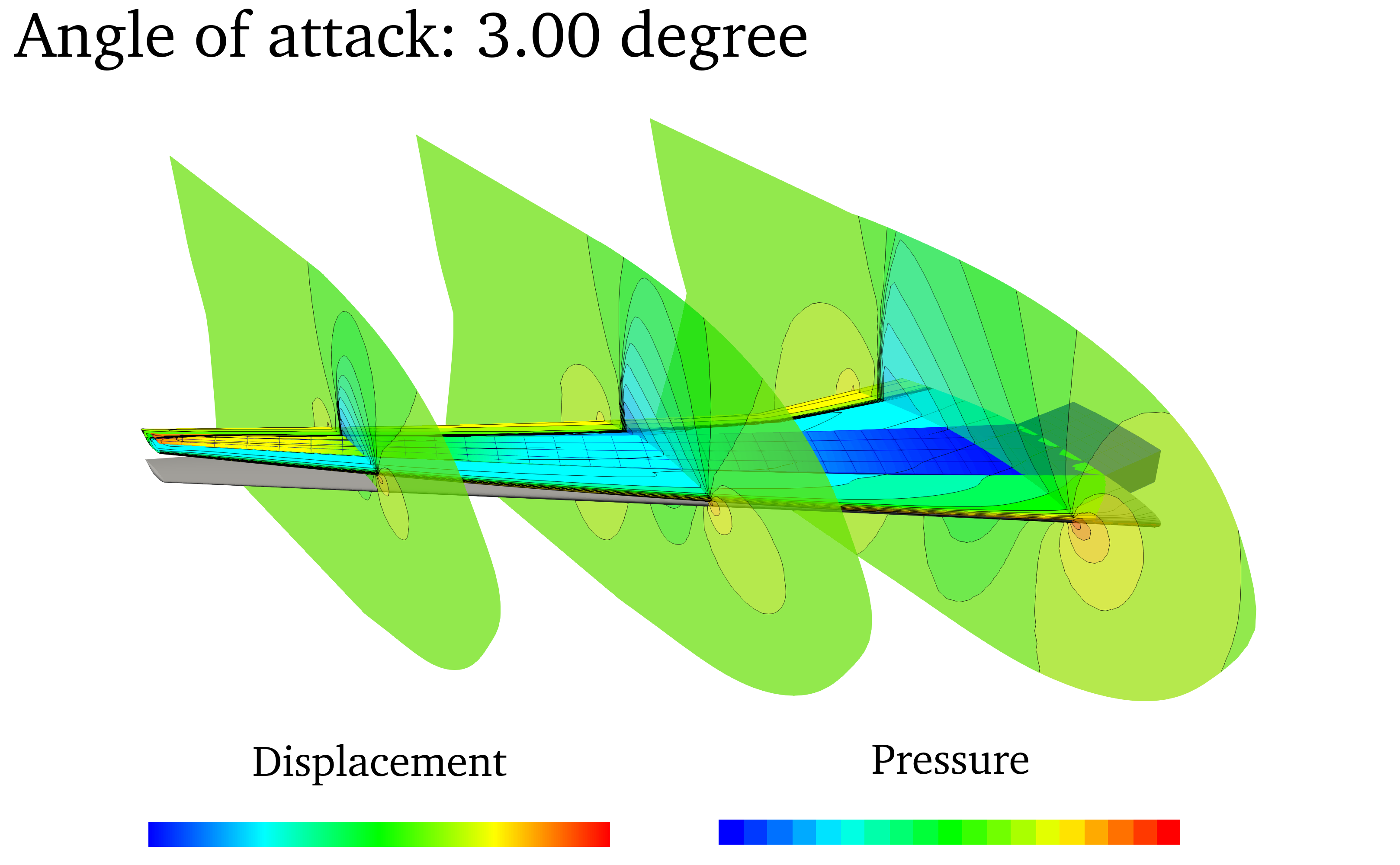
Aeroelastic analysis

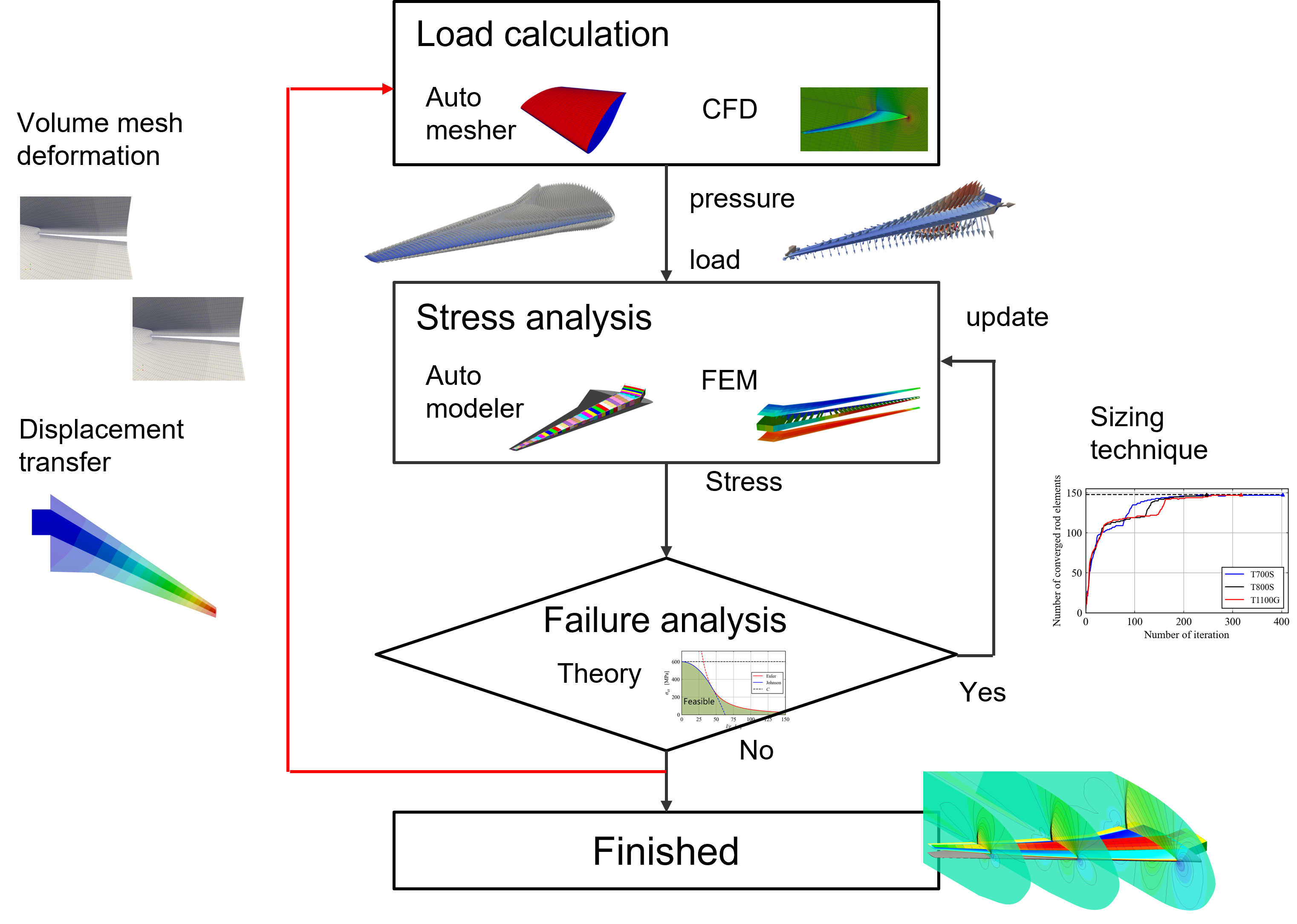
This is a tutorial for performing a two-way coupled fluid-structural analysis.

1. Set your environment

First of all, set work directory in “envs.sh”

#!/bin/bash
set -eu
Pwdir=$(readlink -f .)
OrgDirPath=$(readlink -f .)
WorkDirPath=${Pwdir}/"NAME_OF_WORK_DIRECTORY"
...

2. Set input files

Input files are set by default. If you want to change the analyisis condisions, model, solver, or algorithm, edit the following files.

Edit “system.sh” for a comprehensive setting of analysis conditions, e.g., solver, algorithm, number of iteration.

Data

File

Supplement

Analysis system

system.sh

Edit a list of files to change a wing model.

Data

File

Supplement

Wing geometry

Inp/Configs/winggeom.ini

Structural layout

Inp/Configs/stlayout.ini

CFD mesh info.

Inp/Configs/meshCFD.ini

CFD setting

Inp/Configs/CFD/

according to conditions

Material property

Inp/Configs/material.ini

Structural gauge

Inp/Gauge/gauge_minmax.csv

Inp/Gauge/gauge_init_shell.csv

Inp/Gauge/gauge_init_rod.csv

3. Execute analysis

Command is simple to carry out the analysis.
bash main.sh >& "log_file_name" &
Depending on the setting and usage of MPI, the analysis will be terminated in 1-2 hours.

4. Post Process

You can see the results of analysis by opeing visualization files with your own hands. A list of visualizatino file is summerized below. The “File” in the list omits the path to your work directory (in “envs.sh”).

Data

File

Supplement

CFD surface mesh

01CreateFluidMesh/surface01.vtk

CSM model

02CreateStructMesh/wing_st.vtk

CFD results

04CalcFluidForce/CFD/work/results_cfd*.vts

04CalcFluidForce/CFD/work/results_cfd_surf.vts

CSM results

06CalcStructDisp/*G/result_FEM*.vtu

FEM results with *G laod factor

06CalcStructDisp/*G/result_FA.vtu

Failure modes and MS with *G laod factor

06CalcStructDisp/result_FEM*.vtu

FEM results at cruise condition

06CalcStructDisp/result_FA.vtu

summery of failure modes & MS

It is important to check results manually for validation and understanding the physics. However, the process requires a significant amount of time and hundreds of clicks. Therefore, we provide a series of plot programs to automatically generate plots of physical quantity.

Planform Optimization

This is a tutorial for planform optimization using two-way coupled fluid-structural analysis. NSGA2 is implemented as an optimizer, but another optimizer can be implemented at your own.

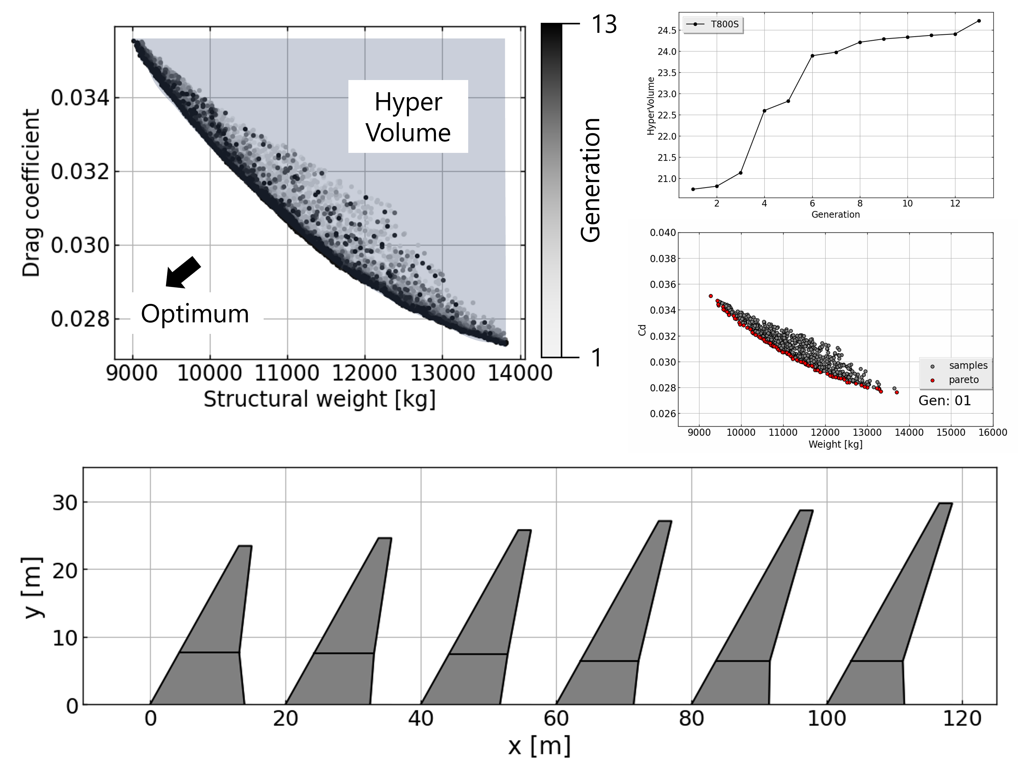
../../_images/plot.png — Objective functions (L), Hyper Volume (UR), Initial (BR), Planforms on pareto plane (B)

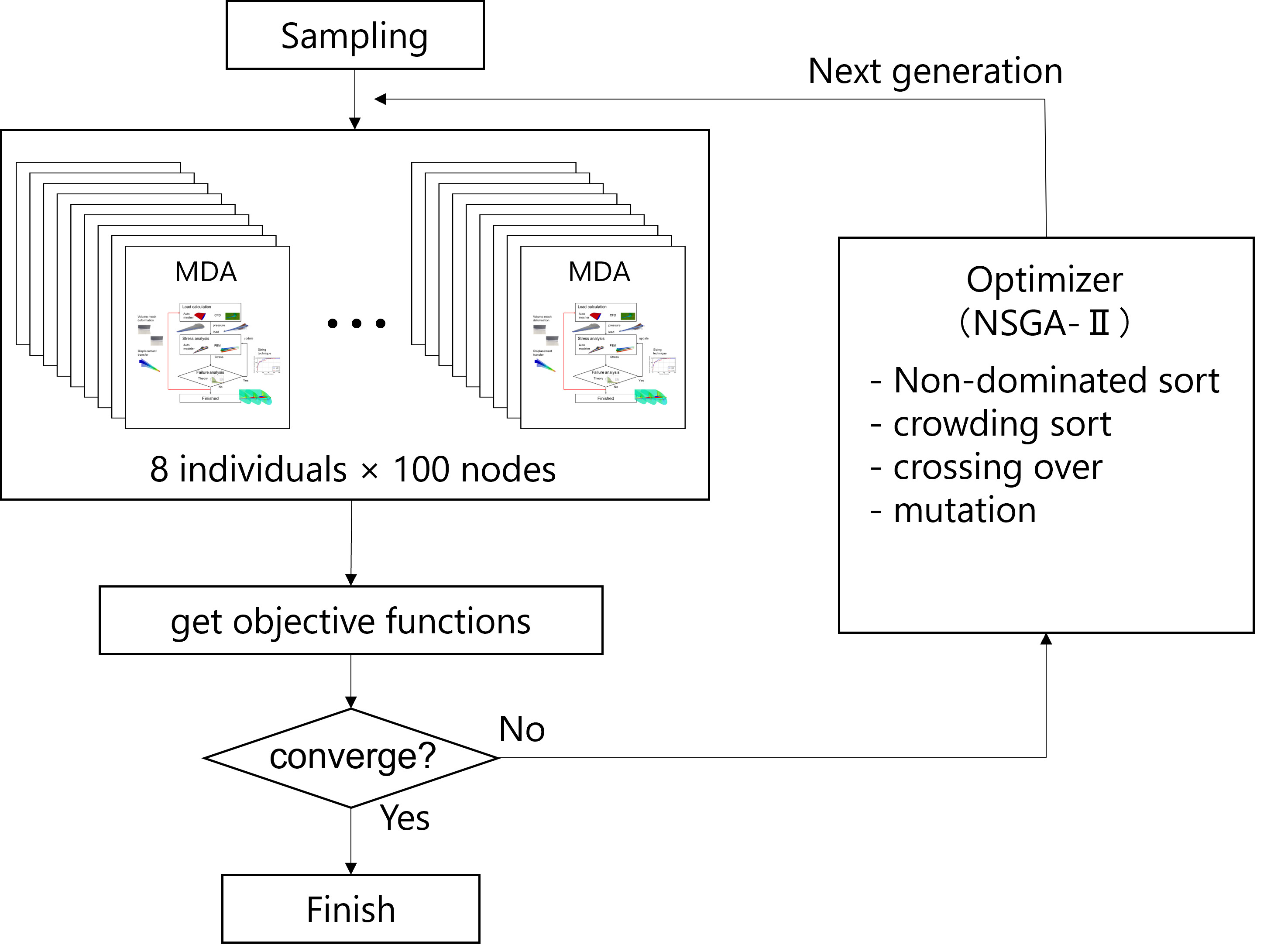
../../_images/flow1.png — Procedure of planform optimization

1. Set your environment

Refer to 1. Set your environment

2. Set input files

Edit “system.sh” for model-wise parallelization. Check the number of parallelization and optimization flag.

In that case, CFD can not be parallelized because we do not use “MPI_Comm_spawn”. Thus, Edit “system.sh” as like this.
# MPI number
NPMAX=8

# optimization problem
OPT_PL='on'
OPT_AF='off'

...

MPI_CFD='off'
Another settings for aeroelastic computation are available in 2. Set input files

3. Execute analysis

Command is simple to carry out the optimization.
bash exec_nsga2.sh >& "log_file_name" &

4. Post Process

After the optimization, work directory may look like this. models* or gen* means generations of Genetic Algorithm. model* means individuals in a generation.

Workdirectory/
├── models0001
│   ├── model0001
│   ├── model0002
│   ├── model0003
│   ├── model0004
│   ├── model0005
│   ├── model0006
│   ├── model0007
│   ├── model0008
│   ├── model0009
│   ├── model0010
│   ├── model0011
│   ├── model0012
│   ├── model0013
│   ├── model0014
│   ├── model0015
│   ├── model0016
│   ├── objs_all.csv
│   ├── objs.dat
│   └── work_nsga2
├── models0002
│   ├── model0001
│   ├── model0002
...

You can see the results of analysis for each individual by 4. Post Process

Ofcource, it is not necessary to check all the tens of thousands of different individuals on your own. The plot_programs in Util automate it for you.

Example1: interactive plot for skimming.

You can check individual differences by moving a mouse.
python Util/archives/iplot_objs.py "your_work_dir"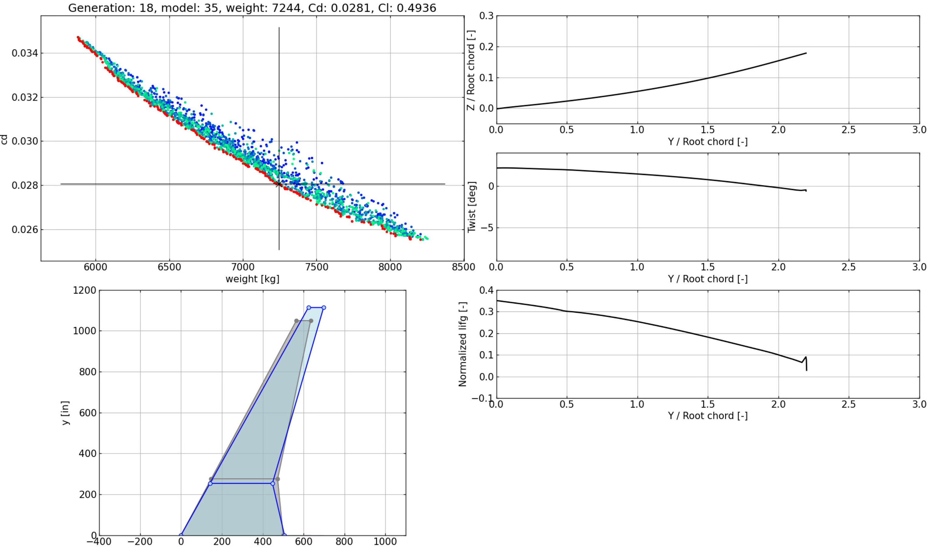

Example2: plot objective functions

python Util/plot_programs/3Dplot_mat.py

Example3: plot correlation of design variables

python Util/plot_programs/plot_corr.py

Shape Optimization

This is a tutorial for shape optimization using two-way coupled fluid-structural analysis. In this document, shape optimization means (planform+airfoil) optimization. NSGA2 is implemented as an optimizer, but another optimizer can be implemented at your own.

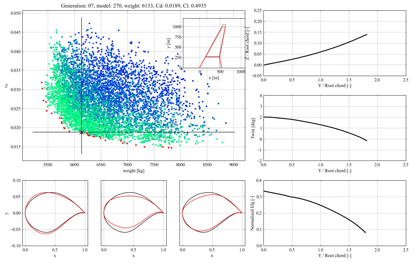
../../_images/plot1.png — Objective functions (UL), Airfoils (BL), Deflection (UR), Twist (MR) Lift (BR)

1. Set your environment

Refer to 1. Set your environment

2. Set input files

Edit “system.sh” for model-wise parallelization. Check the number of parallelization and optimization flag.

In that case, CFD can not be parallelized because we do not use “MPI_Comm_spawn”. Thus, Edit “system.sh” as like this.
# MPI number
NPMAX=8

# optimization problem
OPT_PL='on'
OPT_AF='on'

...

MPI_CFD='off'
Another settings for aeroelastic computation are available in 2. Set input files

3. Execute analysis

Command is simple to carry out the optimization.
bash exec_nsga2.sh >& "log_file_name" &

4. Post Process

After the optimization, work directory may look like this. models* or gen* means generations of Genetic Algorithm. model* means individuals in a generation.

Workdirectory/
├── models0001
│   ├── model0001
│   ├── model0002
│   ├── model0003
│   ├── model0004
│   ├── model0005
│   ├── model0006
│   ├── model0007
│   ├── model0008
│   ├── model0009
│   ├── model0010
│   ├── model0011
│   ├── model0012
│   ├── model0013
│   ├── model0014
│   ├── model0015
│   ├── model0016
│   ├── objs_all.csv
│   ├── objs.dat
│   └── work_nsga2
├── models0002
│   ├── model0001
│   ├── model0002
...

You can see the results of analysis for each individual by 4. Post Process

Ofcource, it is not necessary to check all the tens of thousands of different individuals on your own. The plot_programs in Util automate it for you.

Example1: interactive plot for skimming.

You can check individual differences by moving a mouse.
python Util/archives/iplot_objs.py "your_work_dir"

Example2: plot objective functions

python Util/plot_programs/3Dplot_mat.py

Example3: plot correlation of design variables

python Util/plot_programs/plot_corr.py