
2-D and 3-D Vectorized adaptive solver (VAS2D & VAS3D)
|
first published on November 1, 1997, last revised on August 2, 2007)
In most problems with various length scales, an adaptive mesh
method may reduce the cost of achieving a given resolution by an order
of magnitude or more. However, the method makes it much difficult in
exploiting the resources of a supercomputer. We developed a locally
adaptive code for any structured or unstructured quadrilateral grid
for two dimensions (VAS2D) and hexahedral grid for three dimensions
(VAS3D). The data structure is designed to vectorize the adaptation
procedure as well as the flow solver, without increasing the overhead
on a computer with a single CPU, so that it can be run with a high
efficiency in various platforms, supercomputer as well as a desktop
computer. This page introduces the basic idea behind the VAS2D and the
VAS3D.
Overview
Pre-processing
A quadrilateral grid is automatically generated by an in-house mesh tool or commercial softwares for any desired computational domain. The grid data is then automatically transformed to the cell-edge data structure that is used in the flow solver and the adaptation procedure.
Flow solver
In principle, any scheme that belongs to the family of the finite volume method can be used to treat complicated control volumes. Two schemes have been constructed in the VAS2D. One is the MUSCL-Hancock scheme, a second-order upwind scheme, another is a second-order central-difference scheme with artificial smoothing.
Adaptation procedure
refines flow regions with large numerical errors, and coarsens regions with small truncation errors. The cell-edge data structure is applied to the flow solver and the adaptation procedure. The source code is written in Fortran, about 1,100 lines for the adaptation procedure (greatly simplified from and 500 lines for the flow solver.
Post-processing
transforms data on the cell-edge data structure to the conventional vertex-centered or cell-centered structure, then flow visualization and data processing can be realized by using commercial softwares. The VAS2D provides a few simple but quick subroutines to investigate results, by outputting iso-contours or fringes in the PostScript format; numerical results shown in this webpage (.GIF pictures) are directly transformed from the output of the VAS2D. Post-processing will not be discussed further (although it is equally important).
The source code was originally programmed in Fortran. The adaptation module contains about 1,100 lines for the adaptation procedure (300 lines shorter than previous versions) . A typical module in the flow solver is a few hundreds lines long. For example, the module for inviscid gas modeling using the MUSCL-Hancock scheme contains 448 lines. Main modules included in the flow solver are data reconstruction module (computing spatial gradients), viscous module (computing viscosity & heat conduction terms), two inviscid modules (computing convection terms using two different schemes).
The three-dimensional adaptive solver using hexahedral cells has
been developed in Fortran 90.
Performance on Cray C90
The flow solver used in this test is the classic Lax-Wendroff scheme. The spurious oscillations which numerically appear with discontinuities are removed by an additional conservative smoothing step. The computational efficiency of all algorithms is measured by calculating a shock wave diffracting over a 90 degree corner. The test runs 400 time steps and uses about 10,000 cells (cell number can not be fixed because of adaptation). The memory requirement for the computation is nearly 2mega words. figure shows the CPU time required for main subroutines of the algorithm in one time step. The flow solver uses 70% of the compute time, other time is mainly spent by grid adaptation, geometry update. The geometry update only computes cell volumes and edge lengths. According to hardware statistics, the average vector length is 117.6 (the maximum machine length is 128), therefore the algorithms are well vectorized. The average CPU time requires about 4 microseconds per cell per step. This speed is over one hundred times faster than that conducted in a workstation using upwind schemes with either exact or approximate Riemann solvers. The efficiency is not only due to the vectorizable data structure but also due to the Euler solver, which is a central-difference scheme with the conservative smoothing.
Note: All computations are carried out in Cray C90 in single processor mode.
Cell-edge data structure
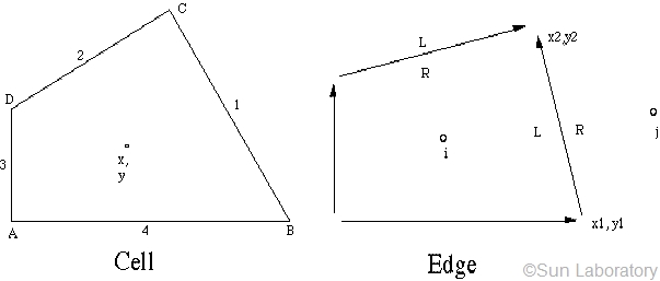
The basic information saved for an edge is the locations of its two ends and the indices of its left and right cells. Note that a cell never directly points to another cell but through their common edge. For instance, if cell i need the information of its right cell j, then it should get the right index of its NE1. It is clear that one adjacent connectivity only needs two memory reads during computation, because of the unique definition of geometry.
Adaptation procedure
The refinement and coarsening procedures are handled separately. Both procedures have similar steps for vectorization:
- handling the inside of cells which are flagged to be refined or coarsened,
- handling the edges of the flagged cells,
- arranging memory.
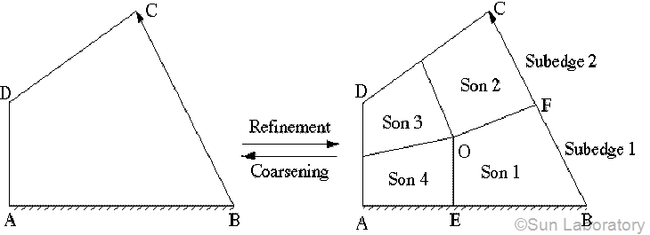
In step 1, it is required that no two neighboring cells differ by more than one refinement level. This rule prevents pathologically large volume ratios under certain circumstances. An illustration of this rule can be found in some literature. A cell to be refined must be divided into four subcells or sons as shown in the Figure. If an edge is split into two subedges, we call the edge a mother, and the subedges daughters. There are some options in the division. One is that the node inside can be optimized to get good shapes of the sons. In present computation the node is set to the center of the father cell. Another option is the locations of new nodes on the outside edges, usually at the centers. But if an edge is a boundary, AB for instance, we choose the new location E so that edge OE is perpendicular to the boundary if this choice does not generate extremely skewed cells. If all four sons are flagged coarse, then they are deleted and recovered to their father cell, which is coarsening.
Step 1 and step 2 change the status of some cells and edges, for example from sons to fathers. Step 3 just cleans and arranges the memory, and divides all cells and all edges into two groups, father/non-father and mother/non-mother, according to their updated statues. The non-mother edges are further divided into boundary/non-boundary edges. These classifications generate an efficient data structure for a flow solver.
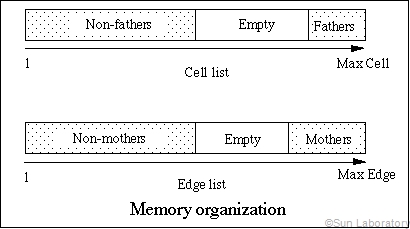
Figure above illustrates memory strides of the edge list and the
cell list after the adaptation procedure. All cell indices are saved
in the cell list, while edge indices in the edge list. Both of them
are constant strides, what vectorization requires. The lists are very
efficient especially for a flow solver using finite volume method.
Non-fathers are just non-overlapping physical control volumes. These
control volumes are numbered consecutively in the cell list. On the
other hand, all non-mothers are all interfaces of the control volumes.
Flux evaluations may be computed along the list of non-mother edges
with vector process.
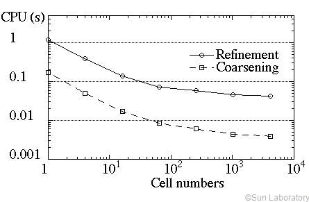
The adaptation subroutine includes 34 loops and about 1,400 FORTRAN
lines. All loops are vectorized. Its practical vectorization
efficiency is tested by refining one cell from level 0 to level 6
(4096 cells), then coarsening the refined cells from level 6 to level
0. Left Figure shows the average CPU time normalized by 10,000 cells.
No flow solver is computed in this test. The CPU time is decreased
with increasing total cell numbers. When the total cells are over
1,000, the speedup is about 30. This indicates that the adaptation
procedure is well vectorized.
Finite volume method
- computing fluxes through non-mother non-boundary edges;
- computing fluxes through non-mother boundary edges;
- computing fluxes through mother edges by adding their daughters' fluxes;
- computing the sum of four fluxes for every cell.
Data reconstruction
MUSCL-Hancock scheme
For the solver using the upwind scheme, the MUSCL-Hancock scheme is applied to unstructured grids. Numerical data is first reconstructed by the least square method at cells, and other procedures are all conducted at interfaces. In slope limiting procedure which aims to maintain TVD conditions around sharp gradients, only gradients in the direction between two neighboring cells beside an interface are modified by limiters. The minmod limiter is used in most applications. The limited slopes at two neighboring cells are then used to evolve solutions at the two cells respectively by half a time step. A HLL approximate Riemann solver is chosen to determine the flux at interface because of its simplicity and generality.
Smoothing TVD scheme
For the solver using the central-difference scheme, a TVD smoothing scheme is used. A predictor step evolves the solution by a modified half time step, by locally solving the two-dimensional Lax-Friedrichs scheme at the interface. Both the interpolation and the predictor step necessitate estimation of the gradients at every cell which are given by the least-square method during data reconstruction. In solving the compressible Euler equations, the fluxes through cell faces, which consist of inviscid fluxes and smoothing fluxes. The inviscid fluxes are convection terms and pressure surface terms, or those in the Euler equations. The smoothing fluxes which are added to suppress spurious oscillations.
References
Sun M. (1998) Numerical and experimental studies of shock wave interaction with bodies, Ph.D. Thesis, Tohoku University.
Sun M. Takayama K. (1999)
Conservative smoothing on an adaptive quadrilateral grid,
J. of Computational. Physics , V150 , pp143-180
Sun M. Takayama K. (2001) A solution-adaptive technique using unstructured hexahedral grids, Anaheim Summer Co-located Conferences, Anaheim, CA, AIAA paper 2001-2656
More Examples
Software for shock wave reflections
Starting Process of a shock tunnel with a hemisphere model
Shock wave diffraction over a 90 degree corner